A simple hydrophone

Here's a blast from my past: a piezo-electric hydrophone. This was my very first research gadget that I ever built. I put it together roughly 10 years ago for my senior research project during either my 2nd or 3rd senior year of undergrad.


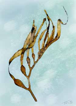
The goal was to listen to predatory whelks feeding on mussels in order to estimate handling time. Because you can't really see the business end (the radula) of a whelk when it's feeding, the only good way to determine when a whelk is drilling is to listen for it.


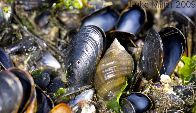
Note the drill holes in the Mytilus edulis shells around the Nucella lapillus shown above.

The hydrophone is based on a piezoelectric noisemaker, commonly found in things like home smoke detectors and Hannah Montana singing greeting cards (Note: it turns out that Hannah Montana greeting cards don't actually contain piezo discs. Stick with smoke detectors).

As sold, these discs make a noise when you apply a voltage across the central ceramic disc and the outer brass disc. But thanks to physics, you can do exactly the opposite as well, produce a voltage across theceramic disc and brass disc by making noise. The hydrophone exploits this property of the piezoelectric noisemaker to turn it into a microphone.

I can no longer find the paper that I read that originally described thissetup, but someone at the Underwater Acoustics Group of the Loughborough University of Technology put together this helpful pdf that describes the construction of the same unit: Acheap sensitive hydrophone for monitoring cetacean vocalisations.

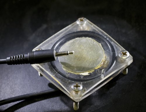
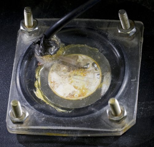
The hydrophone essentially consists of one of these piezo noise makers sandwiched between two pieces of plexiglass, with an o-ring to providethe watertight seal and make space for the wiring.

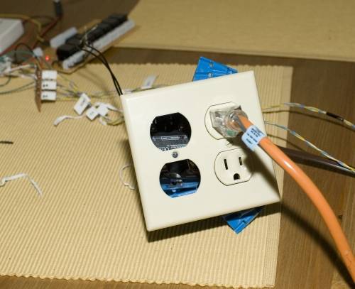
I used a long mono headphone extension cord, as shown in the top picture,for my wiring. The mono cord has two conductors in it. The central conductor gets soldered to the ceramic central disc (visible in the picture above), while the outer conductor gets soldered to the brass disc (not visible above, but see the pdf for a diagram).

The wire is passed through a drilled hole in one of the pieces of plexiglass, which is sealed up with some sort of silicone caulk. 2-ton epoxy might be good here as an alternative.

The other side of the piezo disc then needs to be epoxied to the 2nd piece of plexiglass. This provides a direct connection to the outside world so that sound is transmitted efficiently from the water to the disc. Spread some 2-ton epoxy between the disc and the plexiglass, and let it cure.

The two pieces of plexiglass then get sandwiched together with a thick o-ring (something like McMaster-Carr part number 2418T197) between them to keep water out. The bolts in each corner need to be tight enough to slightly compress the o-ring. In my naive youth I just went ahead and cranked things down until the plexiglass was ready to snap, but it always worked fine.

 

Once everything is put together, you should be able to just plug your cord into the microphone input of a computer and start recording sound. It may be necessary to crank up the amplification quite a bit due to the very low level (low voltage) signal coming from the hydrophone.

When I was actually recording whelks drilling, I found that it helped to use some 2-ton epoxy to glue one of the valves of the mussel directly to the outer face of the plexiglass, right on top of the piezo unit. When a whelk started drilling the mussel, this transmitted the drilling noise(more of a scraping noise really) directly to the hydrophone, helping itstand out from the background noise of water moving through the seawater system. This same system could be glued to a rock to listen to the grazing sounds of herbivorous gastropods. Just don't do anything lame like listen to whale songs. Study something interesting that doesn't have a backbone!

The Marine Ecology Tree

Hot on the heels of the Biomechanics academic tree (described here)comes the Marine Ecology family tree. Like the other trees being built at Academictree.org, the Marine Ecology tree is a user-generated attempt to create an interconnected lineage of professors, graduate students, postdocs and other folks studying marine ecology, or other related fields.

 

Above is the (very incomplete) tree branching off from G. E. Hutchinson. It's up to the users of the site to fill in the (many) missing branches here,and for all the other ecologists on the tree. Eventually this will be a fun resource for anyone wishing to know just how inbred their little section of science really is.

The Biomechanics Tree

Many people have dedicated many decades to studying the biomechanics of trees. Thanks to the people at Academictree.org,the tables have now been turned, and we can finally waste time studying a tree of biomechanics.

Visit the BiomechanicsTree

The Biomechanics Tree is a database of biomechanics researchers past and present. It is your typical academic family tree, showing lineages from advisors to graduate students. You can search for a person and see all of their academic "children" and all of their academic "parents". Masters, PhD, and postdoctoral advisors can all be listed.

The Biomechanics Tree was launched in September 2009, so it's still young. If there's someone missing, create yourself an account and start filling in the missing branches. The tree is user-created, and it's up to the users to make it complete.

As an example of how the tree works, here's a tree centered on Mark Denny at Hopkins Marine Station:


You can see his various graduate students and postdocs on the branches below Mark, and Mark's PhD advisor (John Gosline) and postdoctoral advisor (Bob Paine). Gosline's PhD advisor, Stephen Wainwright, sits on the highest branch here.

If you click on Wainwright's name, you get a tree centered around him:

This tree is quite a bit more extensive, and only part of it fits in the picture here. You can adjust the number of levels of "generations" above and below each person (only two generations are shown here).

Since not ever biomechanic in the world shares the same lineage, there are multiple trees. You can be taken to a different tree by hitting the "Tree" link at the top of each page at the site.

Additionally, if you click on the "Info" link below each person's name, you will be presented with additional information about that person (as available) including their area of study, web pages etc.

There are a number of other academic trees at Academictree.org,including trees for Neuroscience, Drosophila researchers, Linguistics and so on. Keep an eye out for an ecology tree sometime down the road...

Surprisingly, it all works...

I've spent the last few months assembling a conglomeration of parts toset up a new experiment in lab, designed to assess the effects of altered environmental temperatures on snail performance. The goal is to provide these rocky shore whelks with a set of environmental conditions that is as realistic as possible within the confines of a mesocosm, and then augment the ambient temperatures in a subset of the mesocosms.



The snails get to experience the same tidal cycle as in the field, using the local Boston Harbor tide predictions. When the ocean tide drops below the "shore height" of the mesocosms, the tide in the mesocosms drops as well. During high tide, the mesocosms fill with water. The whole setup gets a normal day/night light cycle, since it's outside, andgets exposed to the midday and afternoon sun, similar to a west-facing intertidal site. Temperature increases are accomplished using water heaters at high tide and infrared heat lamps at low tide. Catherine Matassa and her elves (Sarah, Tania, and Nels) helped build the mesocosms that the snails call home.


The setup took a whole lot of custom doohickeys to make it work. Temperatures are continually monitored and power output for the heaters is modulated to produce the desired temperature increase using the circuits pictured above.


A computer runs everything, records data continuously, and evenoccasionally posts updates to Twitter so that I can keep tabs on what's happening in lab even when I'm not there.




We'll have to wait and see what all this produces in the experiment down the road.

Your boots are stupid

These are the best boots for working on the shoreline. Your boots are stiff and uncomfortable. These boots are pliable and more cushioned than your mattress. You should switch to these boots. It's that simple.

I buy them here:ServusXtratuf Steel toe 16" boot at Seattle Marine.
SKU: SRV22271G

If you don't want a steel toe, these are the regular model: ServusXtratuf regular 16" boot.
SKU: SRV22272G

They all run 1 size larger than regular shoes. I buy a size 12. They're better than your boots.

Twittering BBQ

My barbecue has its own Twitter account. If you want to follow along when I smoke some brisket or fish, hit up http://twitter.com/lukesbbq.Please understand that this account will send out an automated update every 30 minutes when I'm cooking, so the novelty may wear off quickly. Below is a description of how I set this up.


This is my Brinkmann "Gourmet" Electric Smoker. It is a decent piece of kit in stock form, but it does let the internal temperature climb too high quite often. The heating element is an unregulated 1500W electric element that is simply "on" all the time. On a warm day, this can bring the smoker temperature above 250F, too hot for proper barbecuing. I setout to cure this issue by controlling the power to the heating element in order to regulate the temperature of the smoker.

The easiest way to do this is to cut power to the heating element when the smoker temperature exceeds some preset limit, and turn it back on when the smoker cools off. I accomplished this using a relatively expensive solution, but it's what I had laying around.

Measuring temperature
The first step is to monitor the temperature in the smoker. I had purchased a pair of digital thermometers with probes that are meant to be inserted into your meat all the time.

Taylor makes a variety of digital thermometers that all use the same stainless steel temperature probe (seen in the package on the left). These thermometers are available at many outlets (I found mine at Target and a local grocery store) and come in a number of models at different price points. The cheap models use the same stainless steel probe with 4' silicone cord as the more expensive thermometer/timer units. The probe itself contains a thermistor, a resistor that changes its resistance based on its temperature. This thermistor can be wired into a Wheatstone bridge to produce a voltage that varies with the temperature of the probe. I elected to monitor the temperature by building a Wheatstone bridge with 3 resistors (47k ohm) and the probe as the fourth leg. I powered this bridge with the 5 volt supply provided by a National Instruments USB-6008 Data Acquisition Card. I then read the voltage from the thermistor bridge using one of the analog input channels (in differential mode) on the USB-6008.

Basic wheatstone bridge schematic


In the final version I ended up using three temperature probes, so I put three Wheatstone bridges on the little perf board below. The output from each of the three bridges is run to a separate analog input channel on the USB-6008. To get the temperature probes out to the BBQ, I made extension wires that run from the perf board to the patio, where the temperature probes plug in and get inserted into the BBQ.




The output of the temperature probe/wheatstone bridge setup needed to be calibrated in order to produce a temperature. I did this by placing the temperature probes in a beaker of water alongside an alcohol thermometer. I slowly heated the water, watching the thermometer temperature and recording the voltage output from the temperature sensor. By plotting these data in Excel, I produced a relationship between sensor voltage and temperature in Fahrenheit using a 3rd order polynomial. This is accurate to better than 1 degree F over the range of 0 to 212F. Each of the temperature probes from the three different models of Taylor digital thermometers is interchangeable, since they all use the same thermistor in the probe (they have a resistance of ~166k at0F, and around 50k at room temperature).

Controlling the heater
Now that I know the temperature in the BBQ, I can now use the same USB-6008 DAQ to control the power to the heating element in the BBQ. This is accomplished by using a digital output line from the USB-6008 to control a relay that supplies power to the heater. The TTL digital signal from the USB-6008 by itself is not sufficient to power a relay though, so the TTL signal is first fed to a ULN2803 Darlington array. The ULN2803 takes a digital signal from the USB-6008 and switches powerfrom a 12V power supply to drive the coil of a relay.


The relay control board can be seen in the background next to the wheatstone bridge board. The 12V DC power controlled by the ULN2803 is fed to a 2-gang electical outlet box that houses a solid-state relay and a 120VAC electrical outlet, seen below.








The 2-gang box holds a Kyoto KD20C75AX solid state relay. This unit can be controlled by a 4-32V DC signal, and will happily control a 120VAC load of up to 75 amps peak current draw. The 75A peak rating might be overkill for what should be a 12.5A load from the heating element (1500W/120V = 12.5A), but the relay definitely gets hot to the touch running this load.

The electrical outlet on the right side of the 2-gang box is wire to an extension cord that runs to the mains power. Instead of wiring this extension cord directly into the outlet, I ran the hot leg through the solid state relay to control power to the outlet. By doing this, the outlet (and anything plugged into it) are switched on and off by the USB-6008. As shown above, I plug in an extension cord to run out to the BBQ.


The view inside the BBQ shows a roast with the temperature probes inserted into it for this test. Normally one of the temperature probes is mounted so that it hangs in the air in the upper portion of the BBQ, monitoring the air temperature. The other two probes can be put into whatever I'm cooking.

The program
With all of the hardware setup, the last piece of the puzzle is the software that will control everything. I used Labview 8.2 to build a simple program to monitor the temperatures and control the power to the BBQ.

The program monitors air temperature several times per second. The current air temperature is compared to the upper and lower air temperature limits set in the upper right of the control panel. When air temperature exceeds the upper threshold, power is cut off to the heating element. When air temperature drops back down below the minimum threshold, the heating element is turned back on. The thermal inertia in the BBQ is sufficient that you don't need to factor in any sort of hysteresis in the program to prevent the heater control from flipping on and off too quickly. The program will also save the temperatures once a minute in a text file should you want to replay the whole cooking endeavor at a later date.

The basic program worked fine, until I saw a post by Jarrett Byrnes at I'm a chordata! Urochordata!describing his newfound ability to post to Twitter from within the R statistical language. It occurred to me that this might be useful for the BBQ, so I went hunting for an implementation in Labview. That led me to a NI Developer Zone Community post about posting updates in Twitter. Unfortunately the code posted there only works in Labview version 8.6 or later, but there was enough information in the example schematic to write my own Twitter update vi. After integrating this into my BBQ control program, I can now have the BBQ post updates to its Twitter account at 30-min or hourly intervals, and send an additional notification when one of the meat temperature probes exceeds a chosen temperature (i.e. >160F).


The twittering (tweeting, whatever) BBQ control program


The Twitter results. The format changed through time as I refined the formatting.


While a twittering BBQ might seem silly, this does act as a proof-of-concept for my plans to integrate a Twitter updating feature insome of my laboratory experiments that run for days or weeks. The Twitter update is extremely easy to implement (see the "Send_Twitter_update.vi" below), at least until Twitter starts requiringa more secure authentication procedure. This can be used to send regular updates to your cell phone via SMS to show that things are running properly or to send alerts when some variable goes out of bounds. The Twitter update vi could certainly use improvements, particularly with how it responds to errors or connection timeouts (it doesn't do anything right now), but the basics are there.

The BBQ control programs and sub-vi's necessary to run them are provided here. They were developed with Labview 8.2.1 and DAQmx 8.9.

The first three vi's will do the basic temperature monitoring, BBQ control, and data recording. The second vi (thermistor_read.vi) contains the parameters for converting voltage to temperature. Those parameters are specific to my setup, and need to be changed for other wheatstone bridge and temperature probe setups. The third vi is just a file initialization routine.
BBQ_temp_regulation_proto_v4.vi
sub-vi: thermistor_read.vi
sub-vi:BBQ_output_file_initialization.vi

The Twitter-updating BBQ control is:
BBQ_temp_regulation_twitter.vi
sub-vi: Prep_Twitter_update.vi
sub-vi: Send_Twitter_update.vi

The "BQ_temp_regulation_twitter.vi" needs "thermistor_read.vi" to run in addition to the two Twitter-related vi's. If you only want a vi to post updates to Twitter, "Send_Twitter_update.vi" will do that on itsown. Just supply it a message, a username, and a password.

Mussel spawning

I made this little animation a few years back when messing around with getting Mytilus californianus to spawn in the lab. Obviously I was successful at some point.

MAGIC isn't real? How can this be?

Someone warn David Copperfield, because the cat's out of the bag: MAGIC isn't real. Maybe this is all one elaborate hoax propagated just to create amusing headlines, but a Korean research team has had a 2005 article in Science retracted by the journal. It turns out that the paper describing their technique, given the acronym MAGIC (magnetic-based interactive capture), was based on missing and/or fabricated data.

Equation numbering Word 2007

So I can find this later: setting up a custom equation in Word 2007 that will generate numbered equations with the equation centered on the page and the equation number in parentheses on the right margin.
OfficeWord Team Blog

Antibodies

FYI for the three people in the world that might care about this. If inally got around to asking Affinity Bioreagents what happened to their MA3-001 Hsp70 antibody that was so effective on various molluscs. It was discontinued in 2006. The info from the customer representative:

"I checked our product files and was able to find information on the monoclonal antibody to Heat Shock Protein 70, the unpurified ascites product MA3-001. This product was discontinued in early 2006 because at that time production was not able to recover good, active antibody that recognized HSP70 by our in-house Western Blot. Because after several attempts we could not produce good product, we were forced to discontinue this clone. At this point we do not anticipate bringing this product back into our product portfolio."

Abandon all hope...